RESOURCES |
Category: Refining
OLI Systems software makes it easy to solve complex chemistry design and operations problems by leveraging our first principles-based models. When accurate and plentiful data is available, OLI Systems’ base models are well placed to provide valuable insights. However, it is often the case when solving real problems data may be missing or noisy. Missing or inaccurate inputs can prevent accurate predictions. Operations specifically are likely to suffer from poor quality or low availability data. This presents a significant challenge for advanced use cases of OLI Systems’ software such as the design of feedback control mechanisms.
To solve problems where data is missing or noisy, all hope is not lost as there are techniques that can be applied to interpret the information that is available to make predictions and estimates where information is not. To explore these techniques, this blog post will discuss a particular example: the continuous injection of scale inhibitor into a pipe given only noise measurements of the relevant quantities (for example, water chemistry).
To attack this advanced use case problem, we will first need to introduce some Machine Learning techniques, in particular:
- Uncertainty Quantification: the numerical estimation and interpretation of unknowns in data.
- Probabilistic inference of missing data: Machine Learning techniques for estimation of data points away from where measurements are available.
- Probabilistic Forecasting: estimation of the possible future values of quantities and how likely these different future values are.
- Automatic Feedback process control: Artificial Intelligence methods for deciding what actions to take given a set of inputs to maximise some form of reward signal.
Following the overview of these techniques, we demonstrate their application to a demonstrative example: the scale build-up in a water pipe. We will demonstrate how inference of missing data (relying on Uncertainty Quantification and Machine Learning techniques) can be used to design a feedback process control that alters the amount of scale inhibitor injected into the system to minimise cost while minimising the impact of scale build up.
Uncertainty Quantification
Uncertainty Quantification refers to the characterisation and estimation of numerical uncertainties. When aspects of a system are not completely deterministic, or are subject to errors in measurement, uncertainty quantification can be employed to understand and consider these errors.
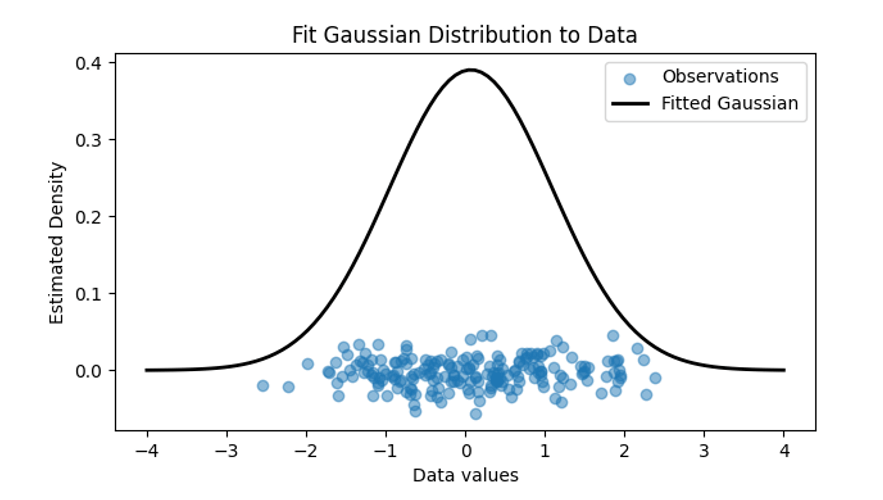
Figure 1: Depiction of noisy observations (in blue) having their uncertainty quantified by fitting a probability distribution to the values with a known mean (central value) and variance (data spread).
To augment a deterministic model of a physical process with an understanding of the uncertainties that are present, one method is to take the deterministic model and ‘push through’ the uncertainties. Uncertain inputs to a model represent a range of possible model inputs (weighted by how likely they are). By passing these ranges of data through the deterministic model, a range of possible model outputs, again weighted by likelihood, is produced. The uncertain outputs represent our best estimate of the true, hidden prediction.
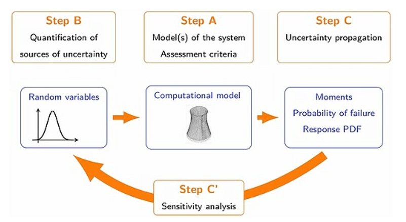
Figure 2: Typical Uncertainty Quantification Procedure (source)
Probabilistic Missing Data Inference
Data may be missing where it is required. If other data is available that is ‘nearby’ in some sense the missing values can be estimated by employing regression techniques. Combining Uncertainty Quantification with Machine Learning gives rise to powerful, probabilistic regression techniques.
For example, imagine taking measurements of scale build-up along the length of a pipeline at regular, but widely spaced, intervals. In-between measurements, how can the amount of scale be estimated? Simple techniques (such as a linear best fit) will fail to consider uncertainties in the data. Gaussian Process regression is one method for making these missing data estimates with quantifiable uncertainties.
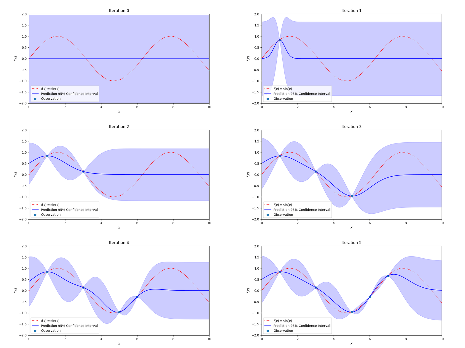
Figure 3: Demonstrating how Gaussian Process Regression becomes more certain of the true, hidden function (in red) with additional observations while also providing estimates of where the true values might be.
Gaussian Process regression uses Bayesian Probability to estimate the uncertainty in measurements over space and or time. Every point over the signal of interest is assumed to be normally distributed and correlated to all the other point-wise Gaussian distributions.
The value of this technique is that pointwise measurements of a signal are augmented with confidence bands that estimate the likely value of future measurements. Close to observations the confidence bands are tight and away from measurements the confidence bands are wide. When new measurements are made, the confidence bands contract down to match the uncertainty in the data. There are other, more sophisticated methods than Gaussian process regression, but they follow roughly the same structure and give similar types of outputs (but may be better suited to a particular use case).
Automated Feedback Process Control
Process control is one of the main areas of Artificial Intelligence research and as applications in fields such as autonomous vehicles and robotics. These techniques can also be employed for the control of chemical plant operations.
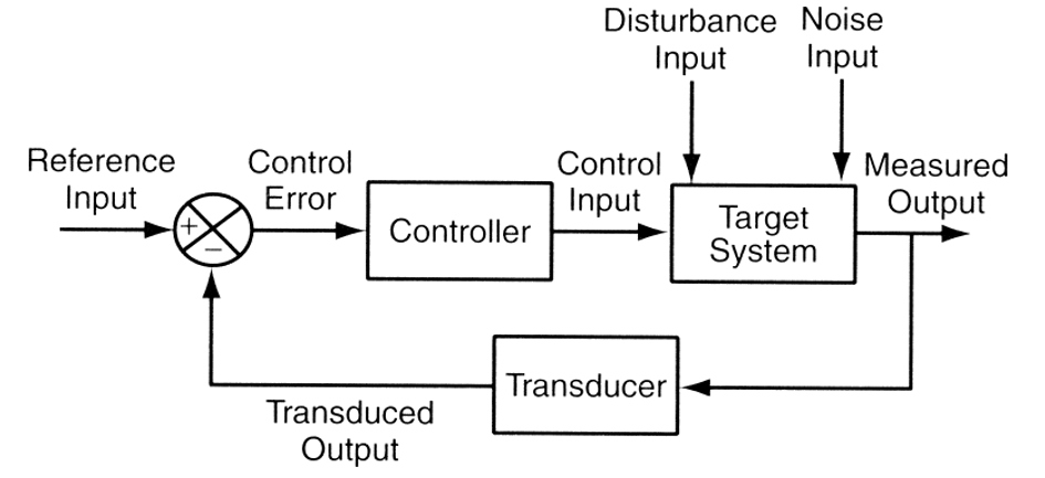
Figure 4: Feedback control system schematic (source)
At a high level, feedback process control requires taking observations of outputs and adjusting some control signal so that the observations are closer to a set point target. There are a broad range of techniques that can be used to design feedback controllers, from PID methods to extremely complicated Reinforcement Learning systems driven by deep-learning including Q-Learning and Deterministic Policy Gradients.
We consider the case of adaptive feedback control systems that modify their parameters over time to better hit their targets. By observing the discrepancy between expected output and the actual output, a difference can be computed that is then fed into a Machine Learning algorithm. The Machine Learning model can learn and adapt to minimise the discrepancy between input and output automatically simply by observing more data.
Example Use Case: Water Scale build up estimation
Consider the case of estimating the amount of scale build-up along a water pipe that is used for transporting brine for industrial operations. Scale inhibitor is injected into the flow stream to prevent the pipe from blocking. The challenge is to minimise scale build-up while also minimising the cost of the scale inhibitor used. In our example, the water pipe is several miles long meaning it is effectively impossible to measure the amount of scale at all possible points within the pipe.
Scale inhibition chemicals are injected into the flow stream to prevent the build-up of solids around the pipe interior diameter which will restrict, and ultimately clog, the pipe. The amount of scale itself is also difficult to measure. Rather, samples of the water are taken and their chemical composition analysed. OLI Systems software can be used to evaluate the scaling tendency of a water sample given the water chemistry.
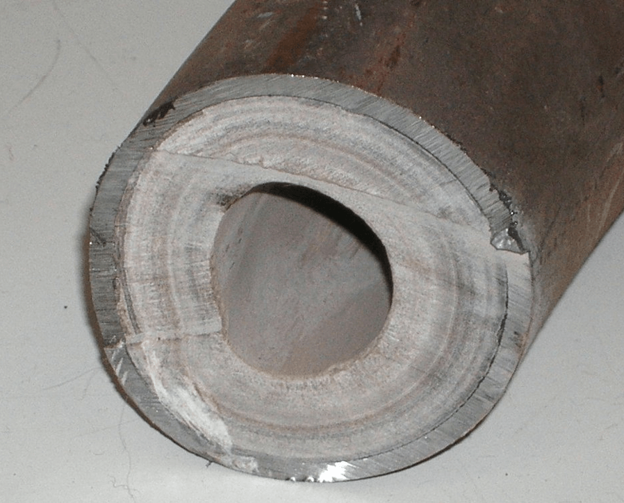
Figure 5: Scale build up in a pipe (source)
The scaling tendency at all points along the pipe can be estimated from a limited set of measurements using Gaussian Process regression. The amount of scale inhibitor that needs to be applied can then be probabilistically estimated to find the minimum dose required to achieve sufficient inhibition. The computed amount of scale inhibitor can then be fed, via computer code, into the control system to alter the dose rate. This forms a feedback loop.
On the next iteration of the system, the observations of the water chemistry are evaluated again. These measurements can be compared against the expected water chemistry targets (given the input amount of scale inhibitor). The discrepancy is calculated and fed into a learning algorithm. In this case actor-critic methods would be suitable. The Reinforcement Learning AI algorithm would predict the amount of scale inhibitor required and continue to learn over time to better predict the amount of scale inhibitor required.
To enhance this feedback loop, Probabilistic Response Surfaces and Forecasting methods based on Machine Learning could be used. This blog post will not discuss these techniques in detail, but will leave this for a future article. The basic idea is that a forecast of the future behaviour of the system is made and the scale inhibitor dose rate is based on the expected future behaviour of the system. Response surface methods can be used to reduce the computational burden of computing the scaling tendency given the input water chemistry.
Advanced use cases of this form are possible today, powered by the OLI Cloud API’s. The full power and adaptability of Python for Machine Learning can be used to develop solutions on top of the OLI Cloud API’s that integrate multiple data sources and compute operationally relevant outputs that improve reliability, safety and ultimately maximise revenue and return. To learn more about this please reach out to us www.olisystems.com/contact-us

